Switched Broadcast

Switched broadcast enables the creation of "virtual" programming capacity without the directly correlated physical expense of creating and dedicating spectral resources. Recent expansions of broadcast programming lineups, particularly those in the bandwidth-hungry high definition (HD) format, have elevated the consideration of a switched broadcast programming tier as a means of providing the capacity to deliver cost-effectively incremental broadcast content. Most practical switched broadcast deployments will (for economic reasons) oversubscribe the number of offered channels to the number of physical stream resources. Thus, a 150-channel switched broadcast tier could be carried on as few as five quadrature amplitude modulation (QAM) channels containing an aggregate total of 50 stream resources. This example configuration assumes that while subscribers may have access to all 150 programs, they will never watch more than 50 different programs at any one time. Much of the value proposition of switched broadcast is tied to the statistical efficiencies that are obtained in specifying this oversubscription ratio. As these statistics are a function of the aggregate viewing behavior and patterns of digital TV cable subscribers, it becomes clear that the support of empirical data would be essential in dimensioning a system. Proof-of-concept trials of switched broadcast were successfully held in 2002 and 2003, demonstrating that switched broadcast services could be carried on existing set-top box platforms and require no modifications to the plant. The success of these trials provided the confidence to support deeper, statistics-focused follow-on trials in 2004, featuring expanded programming lineups and subscriber populations. Figure 1 shows a generic switched broadcast architecture. It includes a broadcast acquisition and transport subsystem, switched broadcast client (SBC), switched broadcast manager (SBM) and an MPEG-aware switch (MAS). Broadcast acquisition and transport subsystem: This can be located in the headend. The acquisition system performs a bit rate clamping function, where incoming broadcast programs are rate shaped to a predetermined constant bit rate (CBR) value. Though not absolutely required, the normalization of all programs to a CBR rate allows a faster and simpler switching mechanism and paves the way for QAM modulator and channel resource sharing with similar services such as video on demand (VOD). The CBR rate chosen most often is one that resembles the program parameters for VOD streams. Using a gigabit Ethernet (GigE) transport structure, the clamped programs are multicast to all hubs. Switched broadcast client (SBC): This is a small software application resident on the set-top box. This client functionality can just as easily be integrated into the tuning firmware of future set-tops. When a switched broadcast program is selected, this software component conveys the channel request via the upstream cable plant, along with information that uniquely identifies the node group location of the set-top box. Switched broadcast manager (SBM): This application runs on a machine located in the hub or headend. The SBM uses the channel number received to identify the requested program, and consequently, the MAS input port where the program is being received. Similarly, the SBM uses the set-top box ID and associates the node group information to determine the downstream connection (MAS output port) where the subscriber can be reached. In many cases, a subscriber can be reached by more than one downstream QAM channel. This collection of one or more QAM channels, and the dozen or so programs that can be carried in each QAM channel, represents a pool of resources that the SBM can use to fulfill programming requests within each node group. When an available downstream QAM channel and the program resource are identified, the frequency and program information are returned via the downstream out-of-band channel to the set-top box, which decodes and displays the program using the normal tuning mechanisms. While the specific frequency and program number for a switched broadcast program may vary in time, the channel number as seen by the subscriber will always remain the same. MPEG-aware switch (MAS): This takes direction from an SBM and connects programming sources with node group destinations. The required switching capabilities can be integrated into an edge-QAM device, or the MAS can exist as a stand-alone entity. System operation The actions that take place when tuning to a switched broadcast program differ from traditional broadcast tuning. In a traditional broadcast environment, all programming is sent via QAM/RF/HFC to set-top boxes, along with data streams that convey the program specific information (PSI) and other channel map information. Using these tables, a set-top box can determine the specific frequency and program number for a TV program and command the set-top box to receive, decode and display the selected program. In a switched broadcast environment, a slightly modified tuning methodology is used. The frequency and program number of any particular program varies in time, and so consequently the content of the tables that carry the frequency and program information for the broadcast channels now vary with time. Therefore, the set-top box uses the out-of-band data channel to acquire the now time-variant tuning information. When this information is retrieved, the tuning process proceeds as normal. To the end user selecting a program via an electronic program guide (EPG) or remote control keypad, this can be designed to be a visually seamless process. Two trials were conducted in 2004 to analyze statistical efficiencies and operational usage of a switched broadcast system. Trial A was deployed in Tyler, Texas, a Cox system. This is a 550 MHz plant using Motorola set-tops and a Pioneer EPG. Trial B was deployed in a 750 MHz system using Scientific-Atlanta set-tops and EPG. Trial B is included to illustrate the effect of increased programming on the switched broadcast tier. (See Table 1.) 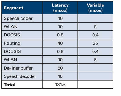Trial A Trial A examined switched broadcast as an alternative to a plant upgrade. The digital channels (already available as a broadcast tier) were simply delivered in a switched capacity. Given the limited spectral capacity of a 550 MHz system, the number of offered programs (60) was much smaller than in Trial B. Trial A was deployed to one node (each node = 1,000 HHP) and later expanded to four nodes. At its peak, 603 digital set-tops were on the switched broadcast tier. Trial B Trial B aimed to conduct a comprehensive statistical qualification and analysis of switched broadcast. As such, the entire digital lineup, minus HD and music channels, was switched. Later in the trial, viewing statistics were also collected for the analog tier. (Though statistics were collected for the analog tier, the analog tier itself was not switched.) Trial B started with a single node containing 334 set-tops, 149 channels of programming and 160 stream resources. Since the number of stream resources initially exceeded the number of offered programs, there was no risk of denial of access for any service. As the trial progressed, the parameters were modified to exercise the system. Three nodes were added to the trial, yielding a final subscriber population of 915 digital set-tops. More programming was subsequently added, growing the switched broadcast tier to 169 programs. Finally, the stream resource pool was reduced from 160 streams (16 256-QAM streams) to 100 streams (10 256-QAM streams). Both trials produced an abundance of log files for analysis. A representative period of time was selected for analysis. In most cases, a one-week period was chosen to comprehensively capture subscriber viewing behavior (weekdays, weekends, etc.). Trial A statistics Figure 2 shows the maximum observed channel use and number of set-top boxes tuned to each channel across a one-week period in July 2004, in 5-minute increments. An important metric to study is the impact of incremental subscribers on the number of watched programs. Intuitively, we know that if more subscribers are added to the switched broadcast tier, the likelihood that they will have different viewing preferences and watch different programs increases. However, it is entirely possible that they will select the same programs as their peer subscribers, which would have no net effect on the number of watched programs. (See Figure 3.) 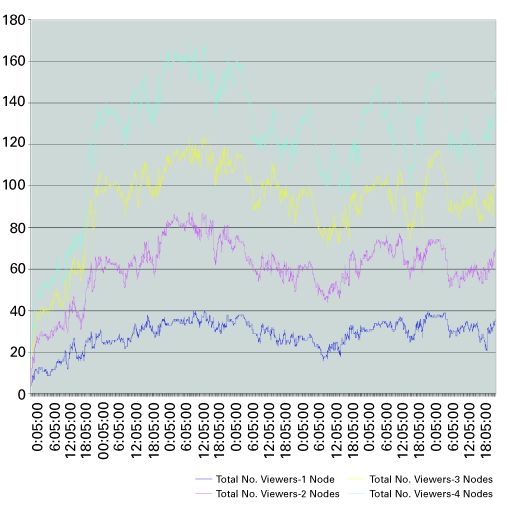Trial A was conducted in four nodes. The granularity of the log files allowed log data to be analyzed on a node-by-node basis. For Figures 2 and 3, data was plotted for node 1, node [1, 2], node [1, 2, 3], and node [1, 2, 3, 4]. This allows the examination of the effects of incremental subscribers on the overall statistics. As is evident from the top plot in Figure 3, the number of set-top boxes simultaneously viewing programs tends to increase linearly as nodes (subscribers) are added to the switched broadcast tier. Note that the gap between the plots at any one point in time remains relatively constant. The impact of additional subscribers to the switched digital tier also has an impact on the maximum number of channels used. Figure 4 demonstrates the increase in peak channel usage across the same period. 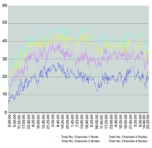Unlike the Figure 3, Figure 4 indicates that as nodes are introduced to the switched tier, the number of channels used tends to increase, but in a logarithmic fashion. Note the gap between the graphs at any one point in time becomes smaller with the addition of each node. The data collected indicates that the channel usage peaked at 50 out of a possible 60 channels. This does not represent a large bandwidth savings, but there are two significant reasons why this occurred. First, when a set-top in switched broadcast mode changes channels, it sends a "tune in" message to acquire the new channel information and a "tune out" message to indicate that it is no longer watching the previous channel. In this trial, "tune outs" from set-top boxes that were turned off were not captured in the data. Hence, the total number of channels used (as indicated by the log file) is artificially higher than normally would be expected. Second, in this trial, the top 60 channels were put on the switched tier. As will be shown in the modeling section later, substantial savings in simultaneous programs viewed are obtained when less popular channels are included in the mix. This is due to the fact that the likelihood of one or more of the less popular channels to not be viewed permits its use by another program. Trial B statistics In Trial B, a large number of programs (171) were put on the switched digital tier. Figure 5 presents the number of channels used across a single day. (One of the busiest days of the week, Sunday, was chosen.) 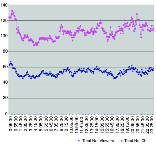On this day in Trial B, the maximum number of channels ever used never exceeds 67, a 60 percent savings in bandwidth use. In this case, both the number of programs and the number of subscribers that have access to the switched broadcast service are greater than Trial A. As expected, the resultant channel use is much smaller as the full suite of programming was included in the switched tier. Unlike Trial A, "tune outs" as a result of powered off set-top boxes were captured in the log file. In this trial, a significantly smaller percentage of the total number of channels, 40 percent vs. 83 percent for Trial A, accounts for peak channel usage. Incremental programming impact Another important consideration in switched broadcast is the effect of incremental programming on the overall system utilization. To study this, the data from Trial B was used. All 171 programs were ranked in popularity, with the number of users and the duration of viewing used as the factors in determining popularity. Then, in groups of 10, the most popular programs were removed from the analysis, and the utilization numbers were recalculated. This process was repeated in groups of 10 until there were no more active programs. (See Figure 6.) 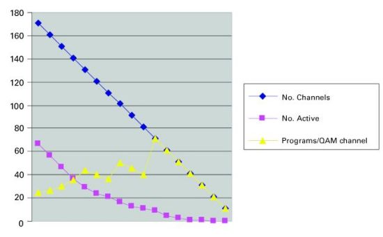The top plot in Figure 6 shows the removal of programs from the analysis. The plot of the maximum number of active programs shows a corresponding decrease. At first, this decrease exhibits a linear pattern with an identical slope. This confirms that indeed the most popular programs are being removed from the switched broadcast tier. As more programs are removed, the decrease becomes more gradual. The final plot of programs/QAM channel in Figure 6 is a rough calculation of the switched broadcast efficiency. Averaged over the entire tier, having more programs per QAM channel represents a higher efficiency. At the start point of the exercise, there are 171 programs available and a maximum utilization of 67. The number 67 is rounded up to 70 (to represent seven QAM channels of available capacity), and we state that for this day, 171 programs could have been carried in seven QAM channels with no blocking. The number of programs/QAM channel is therefore 171/7 = 24.4. Note that this number already vastly exceeds the efficiencies that can be achieved with conventional broadcast techniques such as rate shaping or closed-loop encoding. As programs are removed, the numerator and denominator values change, and the efficiency improves, up to a phenomenally high 71 programs/QAM channel (the least popular 71 programs occupied just nine active streams, or one QAM channel). Since just one QAM channel is now remaining, only the numerator is affected for the remainder of the plot, so the efficiency calculation tracks with the number of programs for the remainder of the plot. Figure 7 shows another representation of the same data. This time, we start from zero and add the most popular programs to the switched broadcast tier, 10 at a time. As expected, the number of active programs initially tracks the number of offered programs. Then, as less popular programs are added to the tier, the number of active programs tapers off. This is a strong visual demonstration of the power of switched broadcast. 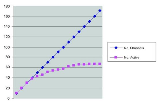Statistical modeling Many manmade and naturally occurring phenomena—including city sizes, incomes, word frequencies and earthquake magnitudes—are distributed according to a power law distribution. A power law implies that small or lower ranked occurrences are extremely common, whereas large, higher ranked instances are extremely rare. In essence, it is a mathematical description of the "80/20" rule. This regularity or "law" is sometimes also referred to as a Zipf distribution. It can be expressed in mathematical fashion as a power law, meaning that the probability of attaining a certain size x is proportional to x t, where r is generally less than or equal to 1. Unlike the more familiar Gaussian distribution, a power law distribution has no "typical" scale and hence is frequently called "scale-free." A power law also gives a finite probability to very large elements, whereas the exponential tail in a Gaussian distribution makes elements much larger than the mean extremely unlikely. For example, city sizes, which are governed by a power law distribution, include a few mega-cities that are orders of magnitude larger than the mean city size. On the other hand, a Gaussian distribution, which describes, for example, the distribution of heights in humans, does not allow for a person who is several times taller than the average. Interestingly, the data obtained in both Trial A and B exhibit a power law distribution that is essentially Zipf in nature in both peak simultaneous use and overall channel popularity. Mathematically, a power law can be stated as follows (Equation 1): pk = Cr-a pk represents the popularity of the k-th ranked item in an ordered list of items ranked by popularity. Note that by multiplying the previous equation by the total number of observations the expected number of each ranked item can be calculated. Hence (Equation 2): Nk = Ar-a Nk represents the expected number of the k-th ranked element. Note that the constant term A will in most cases be different from the constant term C identified in Equation 1. An interesting consequence of either equation is that by taking the log of both sides (Equations 3 and 4): log(pk) = log(C) – alog(r) log(Nk) = log(A) – alog(r) Note that because both of the equations are linear in log(.), both the constant and the exponent term, a, can be obtained by linearly regressing log(pk) on log(r) or log(Nk) on log(r). When using the power law equation to express probabilities, the constant term can theoretically be calculated as follows (Equation 5): K represents the total number of items in the rank order list. In a true Zipf distribution, a = 1. In order to determine if peak simultaneous channel use follows a Zipf distribution, the log of channel popularity—defined as the number of unique set-tops tuned to a given program vs. the log of the rank order of each of the programs, where the highest ranked program (rank = 1) is defined by the channel to which the greatest number of set-tops are tuned—is plotted. Equation 4 indicates that such a plot should be relatively linear. A representative example of one such plot is shown in Figure 8 . 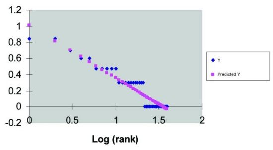The plot in Figure 8 shows the relationship between the two variables of interest for two nodes across the 5-minute period representing the largest simultaneous channel use (that is, widest spread.) Note that the relationship is relatively linear. A summary of the regression output is provided in Table 2. The R2 value, a measure of the degree to which the regression approximation captures the variability in the data, is 0.91, indicating a strong linear relationship. Also of interest are the intercept and the slope of the regression line, denoted as x variable 1, which define the log of the constant term and exponent, respectively. Hence, the estimated equation based upon this data is (Equation 6): Nk = 10.32 * r-0.65 Table 2 also shows a summary of regression analysis for log(channel popularity) vs. log(rank). The same methodology was used to generate Zipf approximations for the 1, 2, 3 and 4 node cases for Trial A. A summary of the results is provided in Table 3. 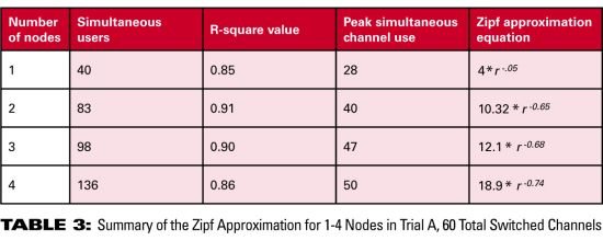Note that the R2 value never falls below 0.85, indicating a relatively strong log linear relationship. Also of note are the Zipf approximation equations whose exponent terms increase in magnitude from 0.5 to 0.74. This results in a greater spread of channel use as dictated by the observed data. The key point here is that an increase in the subscriber base while holding the number of offered programs constant tends to increase the spread of channel usage. This makes intuitive sense, as more subscribers will, in general, create a wider distribution of viewed channels. Both actual and Zipf approximation plots are shown in Figure 9. Note that the approximations do a fairly good job of tracking the overall shape of the observed data. In the samples analyzed, there were several channels to which no set-top boxes were tuned, which could not be incorporated in the log – log plots. Thus, the regression equation tends to overestimate the number of set-top boxes tuned to those channels. 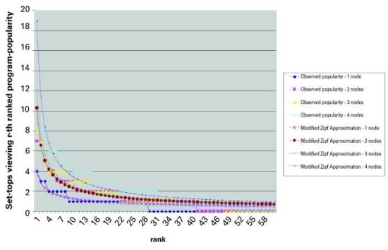Trial B includes the addition of a much greater number of channels, 171, in the switched broadcast tier. The same methodology was applied to this data to obtain the Zipf approximation. Of interest is the peak channel usage as the number of offered programs is increased. We were able to find a 5-minute period in Trial A’s empirical data that contained the highest channel usage and approximately the same number of simultaneous users as a similar observation in Trial B’s data sample. The resulting actual data and associated Zipf approximations are presented in Figure 10. Note that as the number of programs is increased the percentage of the number of simultaneous channels used to the total number of channels offered decreases dramatically. In our sample, Trial A shows that 50/60 = 83.3 percent of the total number of channels is required whereas in Trial B, only 72/171 = 40 percent is required. Note this gain is obtained by adding lower popularity channels to the switched digital tier. 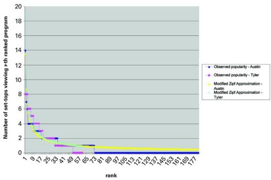This phenomenon is also observed from the Zipf approximation. Table 4 compares the approximation for the relevant data sets of both trials. 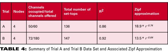Note that the exponent decreases significantly in magnitude in Trial B, thereby tightening the spread of channel use. The approximation tracks the non-zero number of set-tops viewing the r-th ranked program fairly well. However, it tends to overestimate the popularity of the lower ranked programs. Nonetheless, in both cases by using the approximation, a fairly accurate estimate of the total channels occupied can be obtained. (See Figure 11.) 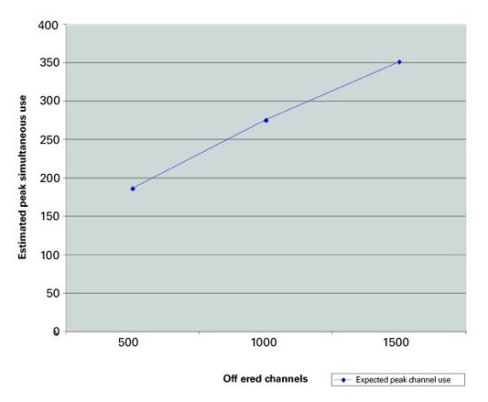Channel usage The previous analysis affords us the opportunity to use a Zipf approximation to calculate the expected channel use if 500, 1,000, or even 1,500 programs were to be offered on the switched broadcast tier. Based on the analysis, the following has been empirically shown: 1) The addition of subscribers (nodes) tends to linearly increase the number of simultaneous set-tops tuned to the view programs. 2) The addition of subscribers (nodes) tends to increase the number of channels used for switched broadcast. However, the rate of this increase diminishes with the addition of subscribers (nodes). 3) Adding programming to the switched service while holding the viewing population relatively constant narrows the channel popularity distribution. This results in a smaller proportion of the total channels offered accounting for a larger percentage of the total views. From this, a Zipf approximation can be used to estimate peak channel use, making the following assumptions: 1) The digital subscriber population and node size is approximately consistent with that observed in Trial B. 2) We chose a very conservative 0.74 value for a as the starting point for 500 channels. This value is considerably higher than that observed in the Trial B data sample with only 180 services. 3) The constant term in Equation 1 represents the popularity of the highest ranked channel (that is, with r = 1.) We estimated this by using ~0.5 of the value obtained from Equation 5, with a= 1. Note that this approximate relationship was observed in the data sets we analyzed. 4) We decreased a by ~0.2 with each increase of 500 channels. Note that this again is a very conservative decrease when compared with the observed data. In our sample, when the channel pool in the switched tier was increased from 60 to 180, a decreased from 0.74 to 0.64. 5) We used the Zipf distribution to estimate the number of channels, K, required to accommodate at least 99.5 percent of total channel use. Note that despite fairly conservative parameter estimates, considerable channel savings can be obtained by putting a large number of services on the switched broadcast tier. A 500-channel system is calculated to require 187 active streams, or 19 256-QAM channels. A 1,000-channel system is calculated to require 276 active streams, or 28 256-QAM channels. And a 1,500-channel system is calculated to require 352 streams, or 36 256-QAM channels. This yields a remarkable ratio of 1,500/36 = 41 programs/256-QAM channel, easily three times the efficiency achievable by even the best closed-loop encoders on the market today. Summary The statistics and subsequent analysis of data from real-world switched broadcast trials have provided a before-unseen insight into the viewing patterns of digital subscribers. Furthermore, a mathematical framework can be fitted to this viewer behavior. This allows the development of tools that can reliably assist in the dimensioning of switched broadcast system designs, as well as assist the development of accurate forecasting of capital needs as switched broadcast systems are expanded. References S.V. Vasudevan and Paul Brooks, "Planning for and Managing the Rollout of Switched Broadcast Services", SCTE Conference on Emerging Technologies, Miami, January 2003. G.K. Zipf, Selective Studies and the Principle of Relative Frequency in Language, 1932. Nishith Sinha is an ITV systems engineer at Cox Communications. Reach him at [email protected]. Ran Oz is CTO and S.V. Vasudevan is chief architect at BigBand Networks. Email them at [email protected] and [email protected].